STEM Solvers

Creating Solver Objects

Starting with STEM V2.0 you can create any one of several different Solver Objects to solve (integrate) the differential equations in your model or models. Choices include:

• Finite Difference
• Runge Kutta
• Dormand Prince 853
• Dormand Prince 54
• Gragg Bulirsch Stoer
• Higham Hall 54
• Stochastic Solver

To create a solver, simply click on the create a new solver icon on the menu bar.

Figure 1: Launching the new solver wizard

The new solver wizard allows you to chose which solver (and which solver algorithm) to use.

For a tutorial on creating and using solvers, please see the step by step tutorial page:  Creating a New Solver

Solvers integrate the differential equations that define models in STEM. In simple terms, a solver determines how the state of a simulation changes from one time step to the next. Models for populations and diseases in STEM are all designed to carry out this change or derivative calculation given a current state. How the derivative is applied to determine the next state is where solvers differ.

Available Solvers

Users can select from STEM Native Solvers or the Apache Commons Math Solvers. The Native Solvers offer speed and ease of use. The Apache Solvers involve more overhead but can offer greater accuracy.

STEM Native Solvers

Finite Difference

The finite difference solver is the most straightforward (and fastest) solver available. STEM's "Finite Difference Solver" is actually better than the fixed time step solution generated by most spreadsheet applications. It uses Euler's method and simply estimates the next value from the current value plus the derivative:

y(t+h) = y(t) +h*y'(t)

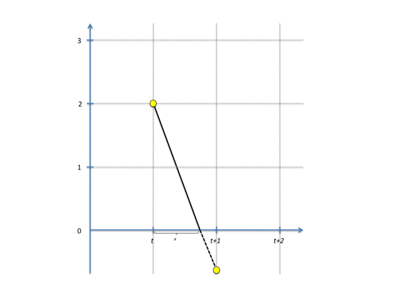
where h is the step size (default 1 day in STEM as defined by the sequencer). Label values in STEM are often constrained to a positive value. For instance, the count of a population can never go negative, and this is also true for any population assigned to a particular compartment state. To prevent constrained values from going negative, the finite difference solver does a partial step to avoid this as illustrated in the figure below:

(the figure assumes h = 1). The next value is thus calculated as:

y(t+h) = y(t) + x*y'(t)+(1-x)*y'(t+x)

The algorithm finds the smallest x among all differential equations solved and rescales all label values accordingly. If necessary, multiple partial steps are carried out. Data is logged (by the loggers) at the fixed time step specified in the sequencer, but if necessary the "finite difference" solver in STEM will dynamically solve your equations at intermediate time steps.

The finite difference solver is able to take advance of multi-core CPUs; each CPU is assigned a sub-set of the graph to work on.

Note: Solvers can only solve valid equations. The finite difference solver has a user configurable "minimum Step"
parameter. If a model is NOT well behaved (due to incorrect mathematics or invalid input data) the solver will stop anytime the step size 
falls below the minimum step and will launch an error dialog reporting the values being generated by the users equations 
so the source of the error can be identified. This type of error condition would only happen if the users model contains an
error causing impossible model conditions (e.g., parameters that diverge or go to negative infinity). The models built into STEM 
all have JUNIT tests and those models are tested nightly (with all of the STEM solvers).

Runge Kutta Cash-Karp

The Runge Kutta Cash-Karp solver is an adaptive step size ordinary differential equation integrator that calculates six function evaluations for each time step and estimates two solutions (of 4th and 5th order). The difference between the two solutions is the estimated error, and the solver can be calibrated to any desired degree of accuracy using the Relative Tolerance parameter. If the error exceeds the tolerance the step size is reduced. The Runge Kutta Cash-Karp solver can take advantage of multi-core CPUs, and each CPU is assigned a sub-set of the graphs to work on. The algorithm perform CPUs synchronization to establish the step size to use, ensuring that the same solution is reached no matter how many CPUs are running concurrently.

For scientific studies where data is being collected for analysis, we recommend using the Runge Kutta Adaptive Step Size method or one of the other numerical integration methods because these algorithms are much more accurate. If you use the Runge Kutta method, you also need to specify a "Relative Tolerance" factor in the disease model parameters. The smaller this number the more accurate the calculations will be, but the simulation will also run slower. The default is 0.05 (or 5%), which we recommend lowering if possible to 0.01 or even 0.001. It all depends how much time you can spare running a scenario.

Apache Commons Math Solvers

These solvers use the Apache Commons Math library and its classes for solving ordinary differential equations. There is some overhead in using these solvers since the STEM data models (graphs/labels etc.) need to be adapted to the APIs expected by the Apache integrators. The advantage to using solvers from this list is that they (especially the Gregg Bulirsch Stoer and Dormand Prince 853) can be more accurate than the STEM Native Solvers. The Apache solvers are maintained and tested independently by the Apache Commons Math community.

Since the 1.4.1 release, all these solvers are able to take advantage of multi-core CPUs to increase performance.

All Apache solvers takes four parameters, Relative Tolerance, Absolute Tolerance, Min Step, and Max Step. Relative and Absolute Tolerance determine the tolerance in the estimated error, indirectly controlling the step size. Min Step and Max Step determine the minimum and maximum step size allowed. If the error tolerance cannot be satisfied by reducing the step size to the minimum allowed, an error is thrown and the simulation stops. The unit of the Max Step and Min Step parameters is in simulation cycles, i.e. one step of the sequencer.

Dormand Prince 853

This integrator is an embedded Runge-Kutta integrator of order 8(5,3) used in local extrapolation mode (i.e. the solution is computed using the high order formula) with stepsize control (and automatic step initialization) and continuous output. This method uses 12 functions evaluations per step for integration and 4 evaluations for interpolation.

This method is based on an 8(6) method by Dormand and Prince (i.e. order 8 for the integration and order 6 for error estimation) modified by Hairer and Wanner to use a 5th order error estimator with 3rd order correction. This modification was introduced because the original method failed in some cases (wrong steps can be accepted when step size is too large, for example in the Brusselator problem) and also had severe difficulties when applied to problems with discontinuities. This modification is explained in the second edition of the first volume (Nonstiff Problems) of the reference book by Hairer, Norsett and Wanner: Solving Ordinary Differential Equations (Springer-Verlag, ISBN 3-540-56670-8).

It is described in the Apache documentation.

Dormand Prince 54

This is another solver from the Dormand Prince family, originally described in:

A family of embedded Runge-Kutta formulae. J. R. Dormand and P. J. Prince. Journal of Computational and Applied Mathematics volume 6, no 1, 1980, pp. 19-26

This integrator is an embedded Runge-Kutta integrator of order 5(4) used in local extrapolation mode (i.e. the solution is computed using the high order formula) with step size control. This method uses 7 functions evaluations per step but since the last evaluation of a time step is the same as the first evaluation in the next time step, one evaluation can be avoided.

More details in the Apache Documentation.

Gregg Bulirsch Stoer

This solver implements a Gragg-Bulirsch-Stoer integrator for Ordinary Differential Equations. The Gragg-Bulirsch-Stoer algorithm is one of the most efficient ones currently available for smooth problems. It uses Richardson extrapolation to estimate what would be the solution if the step size could be decreased down to zero.

More details in the Apache Documentation.

Highman Hall 54

The solver implements the 5(4) Higham and Hall integrator for Ordinary Differential Equations.

This integrator is an embedded Runge-Kutta integrator of order 5(4) used in local extrapolation mode (i.e. the solution is computed using the high order formula) with stepsize control (and automatic step initialization) and continuous output. This method uses 7 functions evaluations per step.

More details in the Apache Documentation

Stochastic Solver

You can run any STEM model stochastically simply by selecting the new stochastic solver. Many infectious processes are by nature stochastic. In a stochastic model, all transitions (e.g. between infectious compartments) are drawn from a discrete binomial distribution (using the Apache Commons math library). As a consequence, only an integer count of humans (or animals) is transitioned from one state to another. This is also what takes place in the real world.

The stochastic solver in STEM takes one input parameter, the stochastic seed. Varying the seed from one run to another will result in a different outcome, and running multiple simulations varying the seed can give you an indication of the range of results possible. If the stochastic seed is the same between two runs, the output of the model is guaranteed to be identical.

known issue: Please note that Stochastic Solvers require that you have a disease model in your scenario (normally you could use STEM to model just a 
population  for example). This  issue only applies to use of a stochastic solver. Even if you are not modeling any disease, the simple fix is to 
create a disease, you can  keep a transmission rate of 0.0, and at it to add it to your scenario. Then it will run fine. 

Incidence of H7N9 avian influenza from a stochastic STEM model of bird flu in China.

Once you have created one (or more) solvers, they will all appear in the solvers folder of the project you are working on. 
Simply drag the solver you want to use into your scenario. Later you can always delete or remove this solver from your scenario and then 
drag in a different one to change your integration method. 

This is very powerful. You don't have to make any changes to your models to switch between a finite difference solver, a
deterministic numerical integration method, or even a stochastic solver!!

Running Stochastic Solvers in Batch Mode

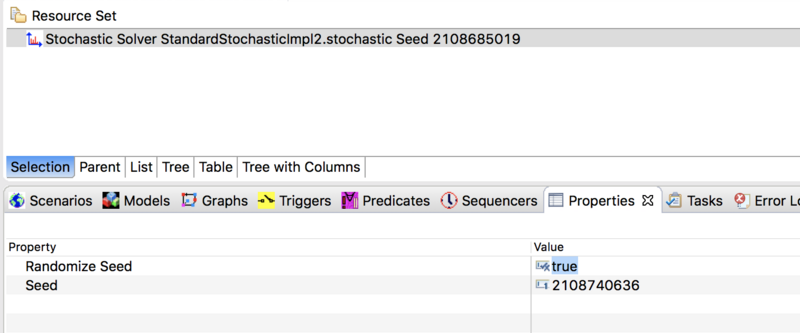
For advanced users who want to use a stochastic solver together with a STEM Experiment (see: Batch_Mode_(Running_Experiments), it is possible to configure your solver to automatically change the random number seed with each execution of your program. To do this, double click on your solver in the project explorer to open it in the resource set. Then double click on the solver in the resource set to open the Properties View. Change the value of Randomize Seed from false (the default) to true. Please observe, if you randomize the seed then STEM will not use the specific seed value set in the properties view but will always pick a new one based on System Current Time (in milliseconds).

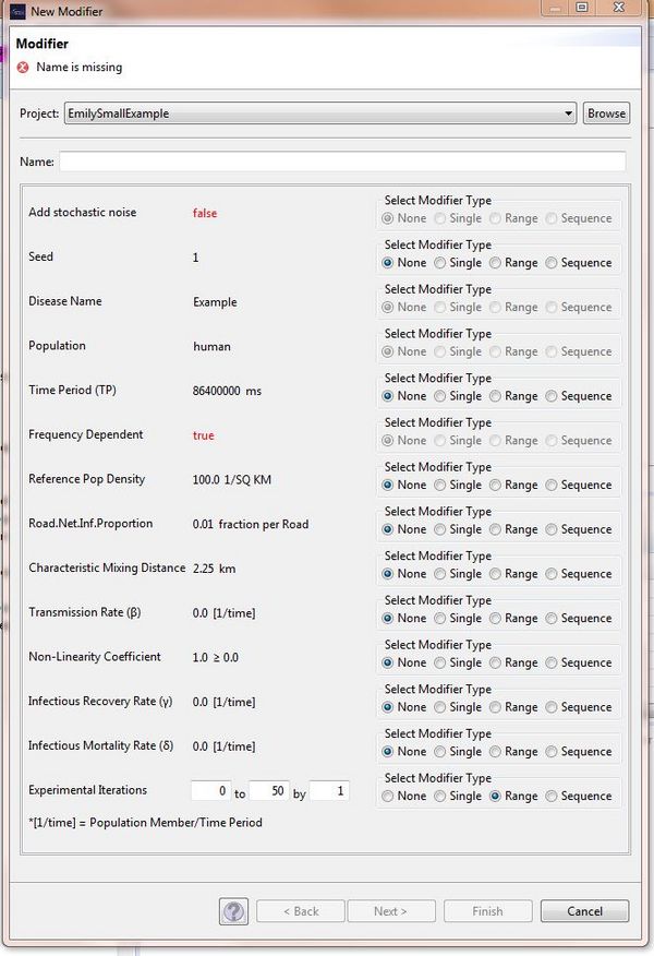
When running your STEM Experiment, you need a modifier which enables the simulation to be repeated for a specified number of times. In order to create the modifier for your STEM, it is necessary to create a new parameter in your disease model which is possible using the Model Creator https://wiki.eclipse.org/STEM_Model_Creator. Once you have created a disease based on your adapted disease model, you can right click on the disease and select "create modifier". You can then modify this new parameter to specify the number of times you would like to run the simulation.

You can see in the image here that the new parameter has been called "Experimental Iterations" and it has been set so that the simulation will be repeated fifty times: