Creating a STEM Scenario

Back

Creating a STEM Scenario

Create the Project

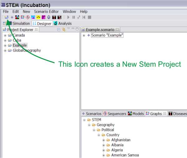
To create a new STEM project, click on the ‘new project’ icon in the command bar, or from the “New”-menu use the “New -> STEM Project” command.

Figure 1: Creating a New STEM Project ("ExperimentalDisease").

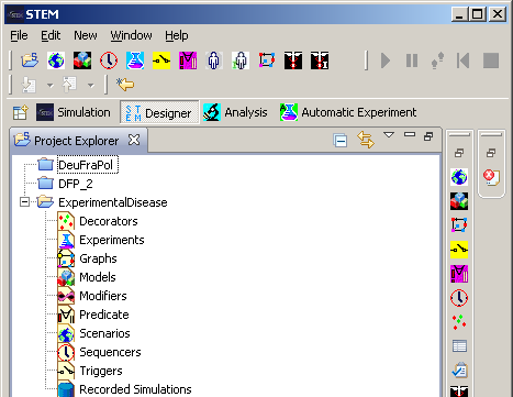
Figure 2: Project Explorer
Give your project a new name, e.g. 'ExperimentalDisease'. The structure created under the new project contains headings for various components, including a substructure for the scenario definitions themselves.

Create a Scenario

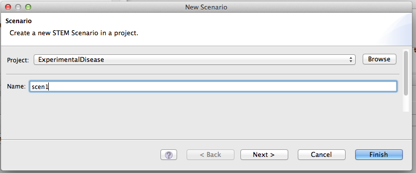
The Scenario is the basic executable unit in STEM. A scenario requires a number of mandatory components to be executable, while some other control elements are optional and can add extended functionality to a given basic scenario. Under the menu item “New -> scenario”, you can create a new scenario entry for the scenarios section of your new project.

Figure 3: Scenario Creation

Starting with Version 2.0 of STEM (October 2013), it is no longer necessary to pick the "Solver algorithm" you want to use. Solvers are now first class objects in STEM so you can easily change your choice of solver without changing your scenario. See the section Create a Solver below.

Create a Solver

With STEM V2.0 and later you can create any one of several different "Solver" objects to solve (integrate) the differential equations in your model or models. Choices include:

• Finite Difference
• Runge Kutta
• Dormand Prince 853
• Dormand Prince 54
• Gragg Bulirsch Stoer
• Higham Hall 54
• Stochastic Solver

To create a solver, simply click on the create a new solver icon on the menu bar.

Figure 4: Launching the new solver wizard

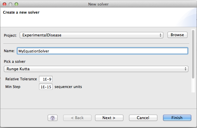
The wizard allows you to name it anything you like. Pick the type of solver you want and click next or finish (if you want to skip the dublin core).

Figure 5: Creating a new Solver

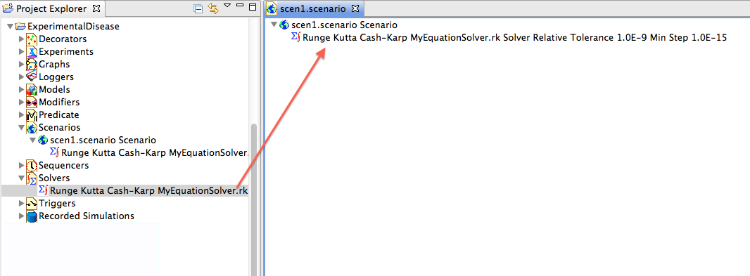
Once you have created one (or more) solvers, they will all appear in the solvers folder of the project you are working on. Simply drag the solver you want to use into your scenario. Later you can always delete or remove this solver from your scenario and then drag in a different one. This is very powerful. You don't have to make any changes to your models to switch between a finite difference solver, a deterministic numerical integration method, or even a stochastic solver!!

Figure 6: Drag your Solver into your Scenario

The Finite Difference method is a simple algorithm that is useful to quickly run a simulation and verify that everything looks right. However, for real scenarios where data is being collected for analysis, we recommend using the Runge Kutta Adaptive Step Size method or one of the other numerical integration methods because these algorithms are much more accurate. If you use the Runge Kutta method, you also need to specify a "Relative Tolerance" factor in the disease model parameters. The smaller this number the more accurate the calculations will be, but the simulation will also run slower. The default is 0.05 (or 5%), which we recommend lowering if possible to 0.01 or even 0.001. It all depends how much time you can spare running a scenario.

For information on the solvers available in STEM, please see the page STEM Solvers

The other numerical integration algorithms (e.g., DormandPrince853, and DormandPrince 54) use the Apache commons mathematical library (http://commons.apache.org/math/) numerical integration methods. For more information on these solvers and what the four parameters do, see the documentation on the library web site (http://commons.apache.org/math/userguide/ode.html).

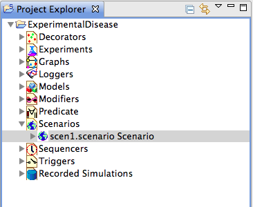
Figure 7: Project Explorer

To be made executable, the blank scenario further requires a sequencer and a nested model structure.

Add Model Containers for the Model Hierarchy

A key concept in STEM is the idea of composing models on top of other models. A model in STEM is a container for graphs; a graph contains nodes, edges and labels. In STEM, a node is typically a geographic region (e.g. France), an edge a relationship between nodes (e.g. the fact that two regions share a common border). Labels store data, for instance the total population of a region or the length of a common border. Models also contain decorators such as disease models or population models. Decorators can create their own labels necessary to store data keeping track of the state of a population. An SI compartmental disease model creates SI labels (on each node) to keep track of the number of susceptible versus infected people in each time step of a simulation.

Models can also contain other models, and this is how you determine dependencies between decorators. As an example, a (mathematical) model of a disease depends on having denominator data such as population data, spatial data (regions), and how regions are connected via common borders, road transportation and air transportation. When something "depends" on something else in STEM, we use nested models to represent such dependencies. A scenario in STEM has a single model (root model if you like) that contains nested models underneath. Deepest down in the model tree you put static data such as graphs containing geographic information (regions with area information and edges representing common borders) and demographic data such as human population counts. This is also where you can place "Population Initializers" to create populations of any type, e.g. animals. On top of this (in the parent model), you can put a mathematical population model describing how the population changes each time step of the simulation. The population model creates the place holders (label and label values) it needs to keep track of the population in each region, and it can also rescale the population initially if needed. This is useful when the population data in STEM (which typically comes from publicly available census data) is not up-to-date with current numbers. On top of the population model (in its models' parent model), you put mathematical models for diseases. Since a disease depends on the initial population numbers calculated by the associated population model (with matching population identifier, e.g. 'human'), it needs to be higher up in the model tree. Finally, above this or in the scenario itself, you create infectors, inoculators or initializers that determines the initial state of the disease (i.e. now many people to infect and where, or what is the background herd immunity).

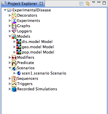
By clicking “New -> model”, you can create an empty model container. In this example, we will need three different models in a nested structure, so we create three model containers, named ‘geo’, ‘pop’ and ‘dis’ for this example.

Figure 8: Model Creation

Import Built-in Models and Graphs from the STEM Library

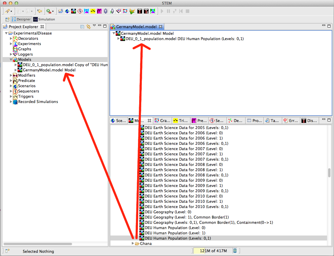
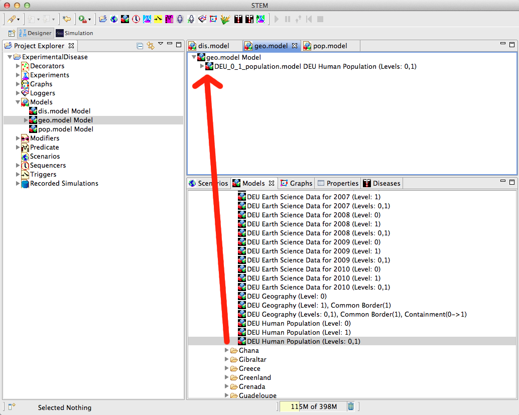
The Models view and the Graphs view (typically located in the lower right corner if you are in the STEM designer perspective) contains pre-built graphs and models you can use to construct your scenario. For convenience, the Models view has commonly used models organized by country. You can select and drag any model from the build-in ones to either the 'Models' folder inside a STEM project, or you can drag it into any existing model part of your project as a child. This screen shot shows both examples:

When you drag a built-in model into a STEM project, a complete (deep) copy of the model is done. This means you can edit the graph using the STEM Graph editor. If you drag a model into another model in your project, only a reference to the model is added and you cannot edit the model.

This particular model contains (DEU Human Population (Levels: 0,1) contains geographical regions in Germany both admin level 0 (Germany) and 1 (German states), the common borders within Germany as well as the containment relationship between Germany and its states. It also contains population data for each state.

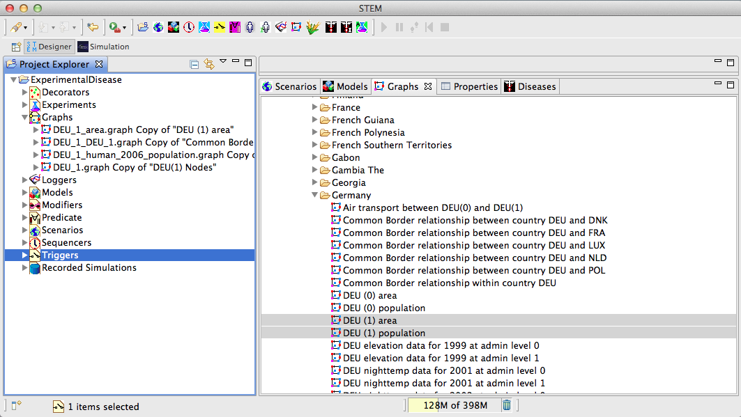
If you want to have more control over the graphs you want as part of your scenario, you can use the Graphs view. Specific geographical data and the population data can be imported as graphs from the STEM library by pulling the graphs from the STEM resources section on the right into the graphs section on the left under project explorer, or directly under an existing model in your project. Here we use country-specific data for Germany.

Figure 9: Graph Import

If you want air transportation as part of your model, you need to select and drag the air transportation graphs from the Graphs view into your model. Air transportation is currently not available in any of the pre-build models.

Create the Geography Model

The bottom model in the model hierarchy is the geographic model. In this case, we will use the pre-build model for Germany human population data down to admin level 1 (states in Germany). This is done by opening the ‘geo.model’ in the Designer view (simply by double-clicking it in the Project Explorer), dragging the model "DEU Human Population (Levels 0, 1)" into the geo.model. Saving your geo.model at this stage is probably a good idea, and can be done by hitting <ctrl S> in the Designer View of the model.

Figure 10: Equipping Models

Create the Population Model

In the model called 'pop', we will store the geography model plus a decorator of type standard population model that grows the population given a background birth rate and death rate. The standard population model is created by opening the "New Population Model" wizard in the toolbar. Select "Standard Population Model" in the drop-down and give it a name (e.g. HumanPopulation). Specify the background birth rate and mortality rate of your population. You also have an option to specify an initial rescaling factor in your population model. You can use this to rescale the population data before running a simulation. This is useful when the population data in STEM comes from census data that's not up-to-date with current numbers. (Currently most census data is from the year 2006 in STEM).

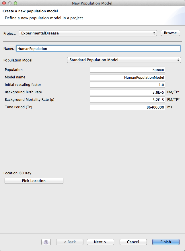
Figure 11: Creating a standard population model

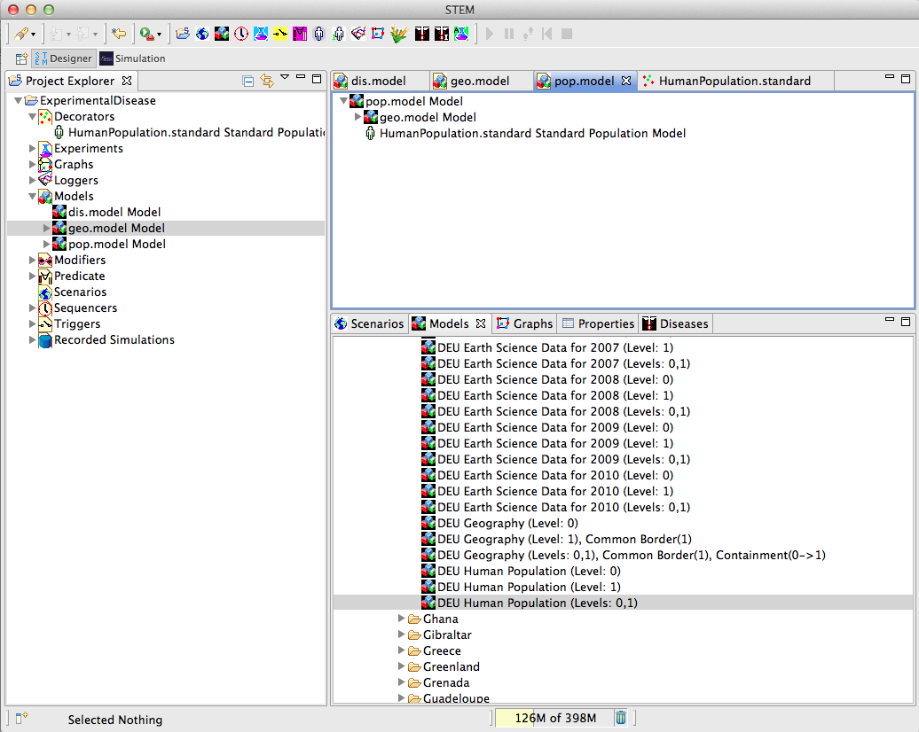
Now open the pop.model in the Designer Perspective, and drag the new standard population model into it (from the Decorators folder). Also drag the geography model (geo.model) from the Models folder in the Project Explorer into the pop.model. Save (Ctrl+S) pop.model.

Create the Disease Model

To compose the disease model, we finally also need a disease. The disease construction is accessible via the “New -> disease” command or by selecting the New Disease Model toolbar icon. For the sake of creating an example disease, note that the transmission rate is set to a value larger than zero, and also note that the name of this disease will be required to initialize the infector later on in the scenario construction. The newly defined disease appears in the ‘Decorators’ section of the Project Explorer, and this is also where the infector will appear when it is created. For this demonstration, we choose a DeterministicSEIRDiseaseModelImpl. with a Transmission Rate of 1.0, an Infectious Recovery rate of 0.5, Immunity Loss Rate of 0.3, and an Incubation Rate of 0.3

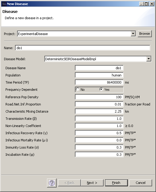
Figure 12: Disease Creation

After creating a disease, you will be able to inspect the properties of the disease in the ‘Properties’ tab of the Resources section of the Designer View. Make sure that all parameters have been entered correctly, e.g. that you have a Transmission Rate larger than Zero. You can change the values of properties in this tab by simply editing them, and saving them by hitting <ctrl-S> in the Designer View again.

To create the disease model, proceed just as before by pulling the pop.model and the disease from the Project Explorer onto the empty dis.model in the Designer View, and save the disease model with <ctrl-S> to update the project.

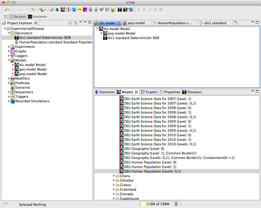
Figure 13: Setting up the model containing the disease

Create an Infector

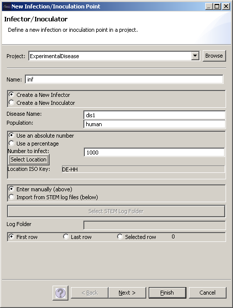
The command “New -> infector” allows you to create an infector, innoculator, or initializer. This sets the initial "disease state" for a given population. Essential information for the infector is the disease to be linked to this infector, thus ‘Disease Name’ must correctly spell out the name of the disease defined earlier. Furthermore, the geographical location must be specified (under the ‘Select Location’ button), in this case Hamburg as one of the 41 nodes in the geographic model for Germany.

Figure 14: Infector Creation

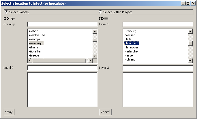
Figure 15: ISO Key selection for Infector

Create a Sequencer

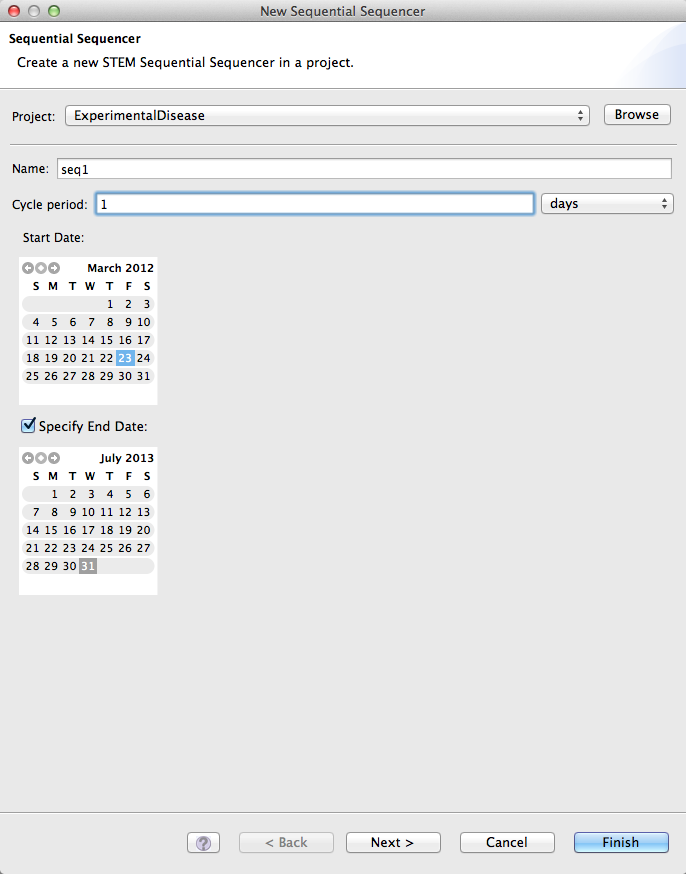
Any scenario will also need a sequencer to be runnable. Under “New->Sequential Sequencer” you can create a sequencer, that specifies the temporal increments upon which the evolution of your scenario will be based.

Equip the Scenario

With a sequencer, an infector, and a nested model hierarchy at our disposal, we can now proceed to equip the scenario. This is done again by simply dragging the components from the Project Explorer onto the scenario heading in the Designer View. The asterisk preceding the scenario name in the tab header of the Designer View indicates unsaved work. Saving the scenario will update the scenario hierarchy in the Project Explorer.

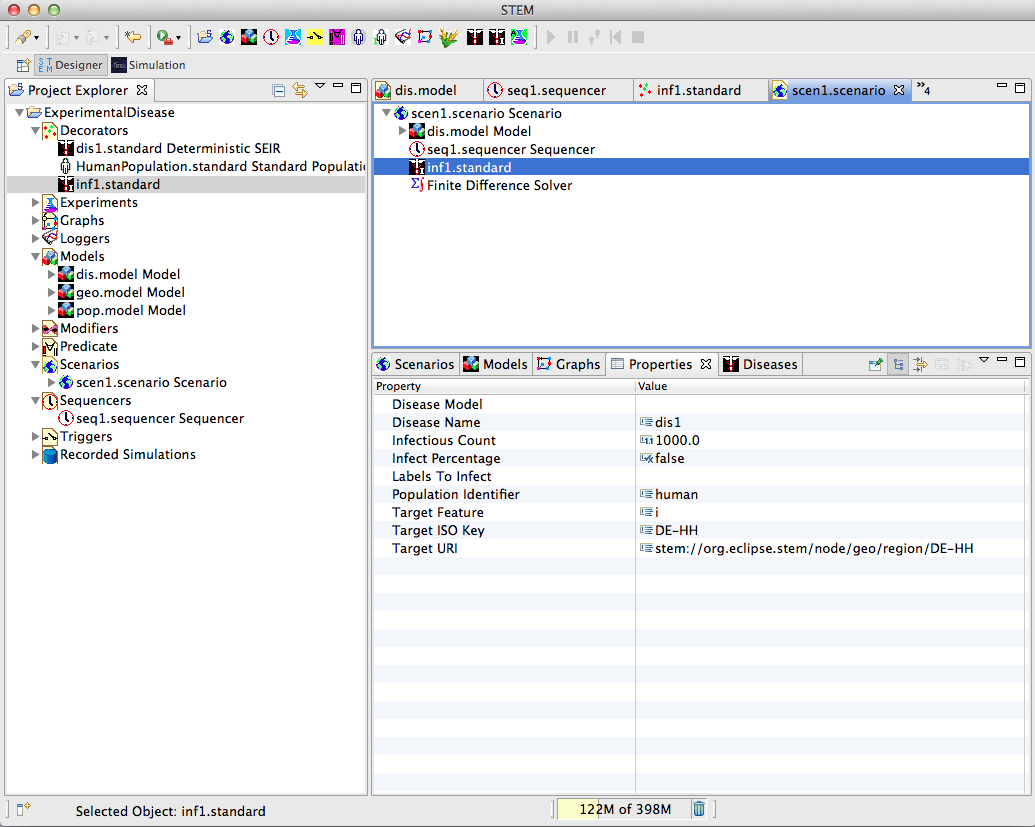
Figure 16: Scenario Completion

Run the Scenario

Right-clicking on the scenario heading and selecting the green triangle icon for “run”, you can now run the scenario and observe the progression of the disease given the selected parameters.

Tips

In case you want to change the properties of a specific decorator in your scenario. Changing properties is only possible in the specific decorator(e.g disease model) under the decorators section in the project explorer. In the STEM models and the scenario is it not possible to change the properties!