Air Travel Model

Introduction

THIS DOC IS IN PREPARATION

STEM contains a model of Global Air Travel that covers 100% of commercial airports in the U.S. and about 80% of commercial airports world wide. The model was calibrated using data on individual tickets within the United States for all of 2007 from the U. S. Department of Transportation Research and Innovative Technology Administration Bureau of Transportation Statistics (RITA-BTS). Tickets give the origin and destination of full trips, rather than individual flights. The RITA-BTS ticket data (DB1BTicket from the Airline Origin and Destination Survey) are a sample of 10% of U.S. tickets from reporting carriers in that year. A complete description of the model is given in the following paper: [http://www.plosone.org/article/info:doi/10.1371/journal.pone.0004403 The Cost of Simplifying Air Travel When Modeling Disease Spread.

The paper describes how we used U.S. ticket data from 2007 to compare a simplified “pipe” model, in which individuals flow in and out of the air transport system based on the number of arrivals and departures from a given airport, to a fully saturated model where all routes are modeled individually. We also compared the pipe model to a “gravity” model where the probability of travel is scaled by physical distance; the gravity model did not differ significantly from the pipe model.

The pipe model roughly approximates actual air travel, but tends to overestimate the number of trips between small airports and underestimate travel between major east and west coast airports. For most routes, the maximum number of false (or missed) introductions of disease is small (< 1 per day); but for a few routes this rate is greatly underestimated by the pipe model.

Methodology

We obtained data on individual tickets within the United States for all of 2007 from the U. S. Department of Transportation Research and Innovative Technology Administration Bureau of Transportation Statistics (RITA-BTS). Tickets give the origin and destination of full trips, rather than individual flights. The RITA-BTS ticket data (DB1BTicket from the Airline Origin and Destination Survey) are a sample of 10% of U.S. tickets from reporting carriers. Using this model we calculated the probability of a trip originating at any airport A, terminating at any other airport B, as

PA,B = TA,B/TA
  

where T_A,B is the number of trips from A to B, and T_A is the total number of trips originating at A. This defines the saturated, point-to-point model.

In order to account for the possibility of flights on unseen routes, we assigned 0.1 trip per year on every possible route not seen in the RITA-BTS data. These non-existent trips account for 0.01% of the trips considered in this analysis.

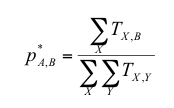
The simplified model we used is a “pipe” model, in which individuals flow in and out of the air transport system based on the number of arrivals and departures from a given airport (i.e., there is no explicit modeling of individual routes). Under this model the probability of a trip from origin A terminating at B is the proportion of all trips at any location ending at B:

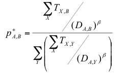
To determine whether differences between p_A,B and p*_A,B could best be explained by the distance between the two locations, we also tested a third “gravity” model of transport. Gravity models have proven useful in general (i.e., non-mode specific) models of transportation [5], and assume that the probability of an individual going from point A to point B is inversely proportional to some power of the distance between those locations. Under this model the probability that a trip from origin A terminates at B is:

We determined the appropriate β for this model by finding the value that maximized the likelihood of the data using a Newton type algorithm (as implemented in the nlm function in the R statistical language) [8]. Note that for a β of 0 this model reduces to the pipe model.

In infectious disease modeling we are interested in the rate of introductions from A to B, λ_A,B, and the overall rate of introductions into a given area, θ_B. Differences in these can be characterized in terms of their ratio, or their absolute difference. The latter is of more interest for the infectious disease modeler, because it can be used to quantify the expected rate of false introductions (or missed introductions) over the course of the epidemic. Table 1 shows these relations. We do not calculate θ_B over the course of the epidemic as this quantity does not have a closed form solution.

All analysis was done using the R statistical package [7].

Comparing the three models

A detailed description of the analysis of all three models may be found online in the paper: [http://www.plosone.org/article/info:doi/10.1371/journal.pone.0004403 The Cost of Simplifying Air Travel When Modeling Disease Spread.

Of interest to the infectious disease modeler is the frequency with which a disease will be introduced under the pipe model, and not introduced under the full model (and vice-versa). To quantify this, we looked at the difference in the rate of introductions from an origin to each particular destination under the two models under the assumption that everyone at the origin is infected with the disease. Using this metric, we found that in only 10% of routes will the rate of introductions be over- or underestimated by at least one person per day, and this over- or underestimation will tend to occur on the most traveled routes. In 2% of routes, the difference in rates is at least 10, and in 0.05% of cases is it at least 100. Only for four routes (JFK→LAX, LAX→JFK, JFK→SFO, SFO→JFK) is the difference at least 500. All of these routes are frequently traveled (≥ 600 passengers a day) cross country routes where the pipe transport model significantly underestimates the probability of the trip (and hence the number of introductions).

While the simplified pipe model of air travel provides a rough approximation of actual air travel, it has several shortcomings. Most of these can be traced back to the pipe model’s overestimation of the number of small town to small town trips. The other simplified model considered, a gravity model which takes into account distance, has similar problems and offers little benefit for the increased complexity.

Underestimation of the number of disease introductions that would occur from travel between major western and eastern populations centers (e.g., Los Angeles and New York) may result in models that underestimate the speed with which the a disease will cross the country. Similarly, the overestimation of the number of locations from which people travel to less busy airports may lead to models where diseases will more rapidly reach locations that might remain protected for a longer period of time. However, for most routes, the size of these effects are relatively small, and the former problem may be correctable by a hybrid model, where frequently traveled routes are treated independently (amplified). Computationally a pipe model offers an enormous advantage as it captures disease transmission by air travel with a 2N edged graph, compared with the pipe model that requires 2N² edges.

The point to point model of air travel also has important short comings. In addition to the computational cost of a 2N² algorithm, a model based on point to point data fails to capture the real mixing that takes place between passengers in the air travel system. A passenger traveling between two major hubs may come in contact with a passenger traveling between two minor locations (possibly through a major hub). This interaction is captured by the pipe model (or a gravity model) but not by a point to point algorithm. Because of its ability computational efficiency, natural mixing characteristics, and good approximation of the point to point probabilities, we chose to implement the pipe model for air transportation within STEM. STEM's architecture also supports the creation of alternative air travel plugins.

The STEM air travel network model

Structure of the air transportation property files

As with other open data, the air transportation model plugin is built automatically by running the "ant" script. Instructions (for developers) for rebuilding this plugin may be found on the page STEM Eclipse Setup. Please see the subsection with instructions on how to Build the STEM Denominator Data. The ant script processes the human readable (and human editable) property files. For air travel these properties files are located in the following folder:

org.eclipse.stem.internal.data.geography.infrastructure.transportation/resources/data/relationship/airtransport2006

within this folder are files containing the data needed to construct a pipe transportation model for air travel. The files have names like:

USA_1_USA_2.properties
and
USA_0_USA_1.properties

The files contain arrival and departure rates based on annual air travel (1996) for 100% of commercial U.S. airports and approximately 80% of commercial airports world wide. The time period for the specified rate is also a parameter in the file and is standardized based on (one day = 8640000ms). The format for the each record is:

# Enclosing Node Key,  Node Key, Arrival Rate (individuals per RATE_TIME_PERIOD), Departure Rate
  (Individuals per RATE_TIME_PERIOD),  Base Node Population.  For example:
# US-AK-02013 =  Aleutians East Borough 
1 = US-AK, US-AK-02013, 22, 22, 2697
# US-AK-02016 =  Aleutians West 
2 = US-AK, US-AK-02016, 40, 40, 5465
...
# US-NY-36081 =  Queens County 
286 = US-NY, US-NY-36081, 46572, 46572, 2229379
...

The arrival and departure rates are equal so the people are not accumulating in the air (and the air travel system is not emptying out). At runtime a user can configure a modifier to change any of these steady state predefined rates. Please see the page on Triggering_interventions#Air Transportation Example. The rates are determined for the annual (2006) passenger traffic through airports within each county (admin 2 region). The air travel node represents the SUM of airports in a county so, for example, Queens County NY is linked to an air travel node representing traffic though both JFK and LGA airports. The rate is the daily rate (annual rate/365 days). The third number (base node population) is obsolete and currently not used.

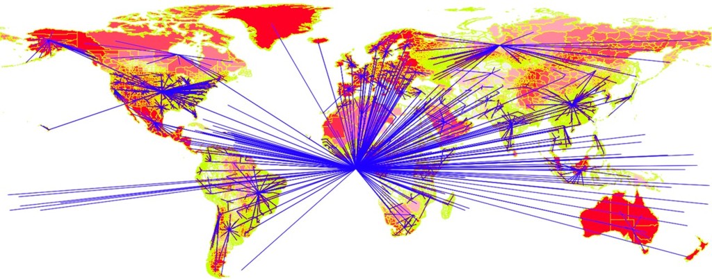
Air travel nodes defined at the county level are connected up to virtual air travel nodes at the state level in a tree structure (e.g. in the file USA_1_USA_2.properties), state level nodes are connect to country level nodes (e.g., in the file USA_0_USA_1.properties), and county level nodes are connected to the international node (in ZZZ_-1_ZZZ_0.properties). As an example, in the Admin 2 (counties) to Admin 1 (state) file for United States (USA_2_USA_1.properties) we have the following entries for air transportation in New York state:

...
276 = US-NY, US-NY-36001, 1977, 1977, 294565 
277 = US-NY, US-NY-36007, 147, 147, 200536 
278 = US-NY, US-NY-36013, 6, 6, 139750
279 = US-NY, US-NY-36015, 114, 114, 91070
280 = US-NY, US-NY-36029, 3455, 3455, 950265
281 = US-NY, US-NY-36033, 4, 4, 51134
282 = US-NY, US-NY-36045, 5, 5, 111738
283 = US-NY, US-NY-36055, 1941, 1941, 735343
284 = US-NY, US-NY-36067, 1546, 1546, 458336
285 = US-NY, US-NY-36071, 215, 215, 341367
286 = US-NY, US-NY-36081, 46572, 46572, 2229379
287 = US-NY, US-NY-36089, 4, 4, 111931
288 = US-NY, US-NY-36103, 1559, 1559, 1419369
289 = US-NY, US-NY-36109, 106, 106, 96501
290 = US-NY, US-NY-36119, 701, 701, 923459
...

Each row is represents the total passenger rate (passengers/day) for all travel, including international passengers as well as domestic passengers traveling to a different state or within New York state. The Admin 1 (state) to Admin 0 (country) file for United States (USA_1_USA_0.properties) has one entry for New York state:

..
14 = USA,US-NY,56368,56368,58352
...

The number specified (56368) represents those travels from NY that are traveling either out of state or internationally, excluding travels within the state. You'll notice that rate (56368) is less than the sum of the rates above (58352), the difference (1984) being the travels within New York state only. Finally, the Admin 0 to Admin -1 (-1 here is the admin level for earth itself) (ZZZ_-1_ZZZ_0.properties) contains the total number of international passengers traveling from United States to a different country:

...
218 = ZZZ,USA,849000,849000
...

Here again, the sum of all rates for US states in USA_0_USA_1.properties is larger than the international passenger rate (849000), the difference being domestic (state-to-state) passenger travel.

Customizing the air transportation property files

Developers are of course free to modify, customize, or update rates in the properties files and can generate a custom plugin by using the ANT script. Rates can also be changed using STEM's framework of modifiers, predicates, and triggers. Users who wish to modify or otherwise generate their own maps in STEM should take note that the current air travel model auto-generates air travel nodes using the same URIs that define the location nodes now in STEM.

If a developer chooses to generate a custom set of maps that adds, removes, or otherwise modifies these URIs, 
then the corresponding nodes in the air travel model must also be updated (as would be the case for 
any 'edge' object in STEM).