Notice: This Wiki is now read only and edits are no longer possible. Please see: https://gitlab.eclipse.org/eclipsefdn/helpdesk/-/wikis/Wiki-shutdown-plan for the plan.
Visualizing Output with ICE
Currently, ICE features three plugins for visualizing and plotting simulation output data:
- VisIt Tools – An interactive 3-D visualization tool for rendering meshes, scalar plots, contour plots, and more.
- ParaView Tools – Another interactive 3-D visualization tool offered as an alternative to VisIt.
- CSV Plotting Tools – A customizable 2-D data plotting utility for comma-separated value (CSV or .csv) data files.
Contents
Prerequisites
VisIt
To use the VisIt tools, ICE requires the installation of Lawrence Livermore National Laboratory's VisIt software (version 2.8.2 to 2.9.2) either locally or on a remote machine.
The VisIt website also offers example data files that you can use to familiarize yourself with the VisIt tools.
ParaView
Using the ParaView tools requires an installation of Kitware's ParaView (version 5.0 or newer).
The user will also need to acquire the ParaView server script (http_pvw_server.py) by contacting the ICE development team.
CSV Plotting Tools
The comma-separated value (CSV) plotting tools are built into ICE and require no additional software to be installed.
Configuring Project Explorer
ICE's "Project Explorer" view allows the user to import data files and launch a visualization session. Currently, ICE supports VisIt, ParaView, and .csv data files. VisIt and ParaView applications are called directly from ICE, and the .csv visualization engine is built into ICE with no need for third-party software.
Opening the Project Explorer View
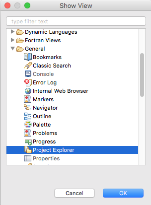
Within ICE, the user will need to have the "Project Explorer" view open. If this view is not yet part of your workflow, use the the main menu bar at the top of the window and navigate to:
Window > Show View > Other
In the resulting "Show View" dialog, select:
General > Project Explorer and click OK.
Creating a Project
The next step is to create a project in which the visualization data files will reside. If you have an existing project into which you would like to import data files, you can skip this step.
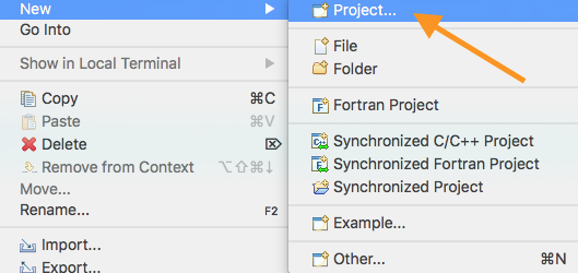
First, right click in the white space of the "Project Explorer" view pane.
In the resulting context menu, select: New > Project.
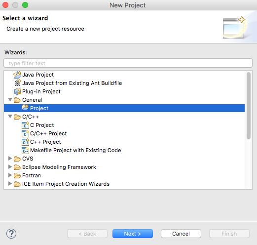
This will present the user with the "New Project" wizard. For this tutorial we're going to select General > Project and then click the Next button.
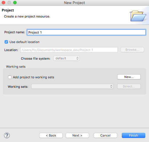
In the next screen of the wizard, create a project name ("Project 1" in this case). You can also choose where to place the project files if you do not want them in the default ICE location.
When you've added your project name and are satisfied with the project path, click Finish.
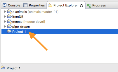
Your new project should now appear in the "Project Explorer."
Adding the Data File
The latest versions of ICE make adding the data file to your project a very simple affair.
First, within the "Project Explorer" view, select the project that you would like to associate with the file you are about to import. In this example, we're looking at "Project 1."
Next, simply click the Import button in ICE's main toolbar.
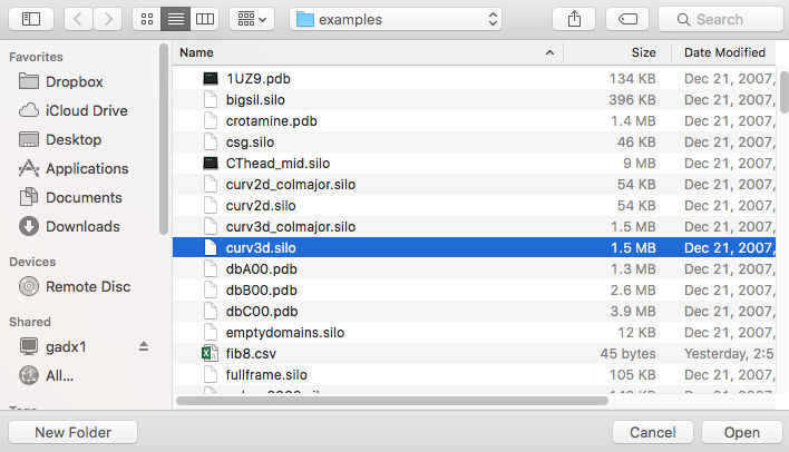
This will present a file import dialog where the user can navigate to the desired data file. Once found, select the file, and click Open.
If needed, you can also select and import multiple files at once.
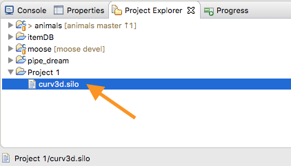
The data file should now appear in the "Project Explorer" view, nested under your project (e.g., "Project 1").
The visualizations for these data files are launched directly from the "Project Explorer" view. For .csv files, you can simply double click their listing in the "Project Explorer" view to open them.
Similarly, VisIt and ParaView files can be opened by double clicking, but you must first establish a connection to the VisIt or ParaView application.
Visualizing Output
Currently, ICE features three plugins for visualizing and plotting simulation output data: VisIt Tools, ParaView Tools, and CSV Plotting Tools. All three plugins, and their implementation within ICE, are described below.
VisIt Tools
Configuring the VisIt Connection
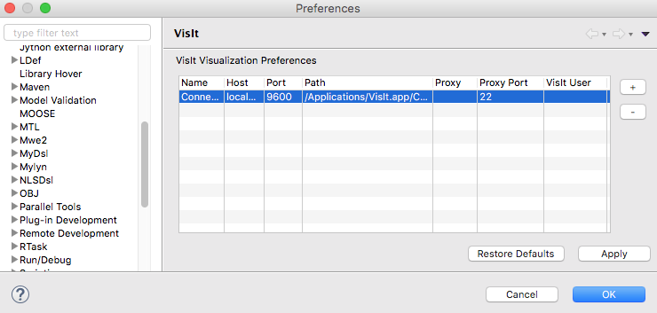
Creating a default VisIt connection will enable ICE to automatically connect to VisIt at launch. To start:
- Windows or Linux: in ICE's toolbar, select Window > Preferences, then Visualization > VisIt in the tree of the "Preferences" page.
- Mac OS X: in ICE's toolbar, select ICE > Preferences, then Visualization > VisIt in the tree of the "Preferences" page.
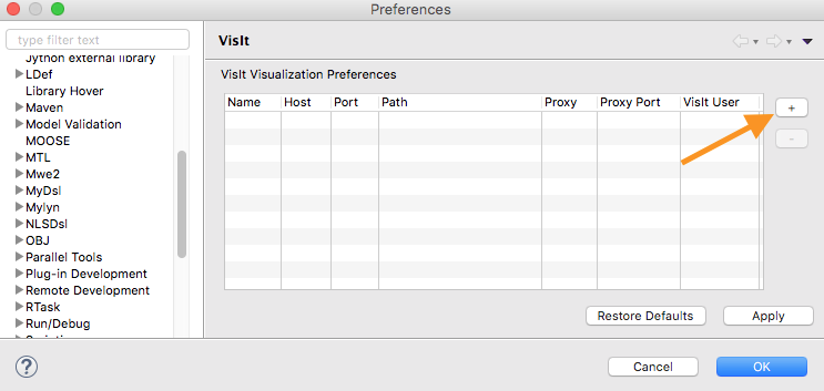
Press the new row button (stylized as a "+" symbol) in the upper-right corner of the resulting dialog box.
The default values supplied automatically by ICE should be fine for most users. However, two fields may need to be changed to accommodate a user's configuration, and you can click on each cell to edit the parameter.
- Host: The default value for this field is "localhost," which is used for connecting to a local installation of VisIt on a user's machine. To launch a remote VisIt connection, the remote hostname/address should be entered into this field.
- Path: If correctly installed, the VisIt path should populate in ICE by default. If not, the user should add the full path to the local VisIt installation. The path should end with the folder containing the VisIt executable.
- On a Windows machine with VisIt installed in the default location, the path would be:
- C:\Users\[UserName]\AppData\Local\Programs\LLNL\VisIt 2.9.2\
- On a Linux machine, the path will be based on where you extracted the visit2_9_2.linux-x86 folder, ending with ~/visit2_9_2.linux-x86_64/bin. For example, if extracted to the desktop, it would be:
- /home/[UserName]/Desktop/visit2_9_2.linux-x86_64/bin/
- On Mac OS X, VisIt should be installed in the machine's "Applications" directory, unless otherwise specified by the user.
- /Applications/VisIt.app/Contents/Resources/bin/
- On a Windows machine with VisIt installed in the default location, the path would be:
Once finished, press Apply, then OK. ICE will then open VisIt and connect to it.
If you are connecting to a remote host, you may be prompted to "allow" the connection to the remote host. Click Yes to trust the connection, and enter the credentials for the remote machine in the prompt.
VisIt Plot Editor
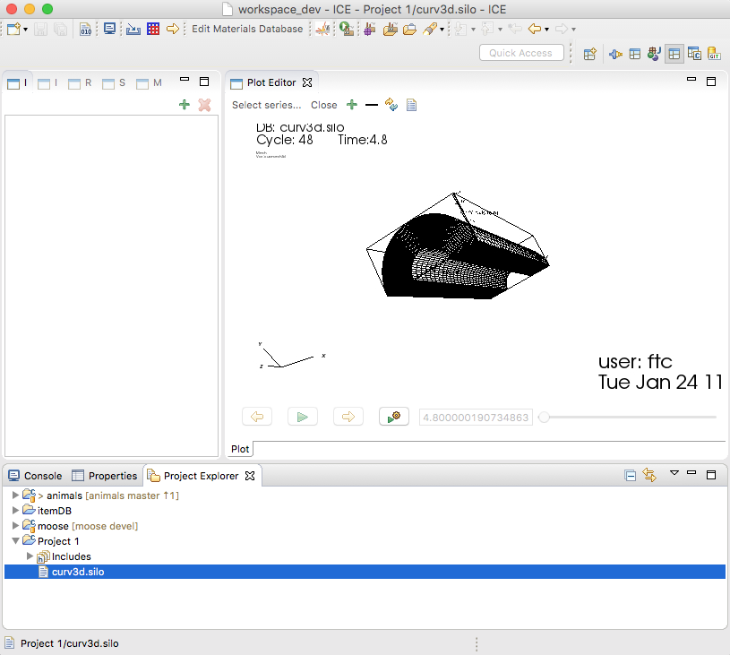
Once a connection with VisIt has been established, the "Plot Editor" view will appear and display the contents of the file that was imported into "Project 1." This view allows the user to manipulate the visualization just as they would with the VisIt GUI.
If at any point you should close the "Plot Editor," simply double click on the imported file to redraw the visualization.
A VisIt plot editor will allow you to choose the mesh and scalar to be modeled and to choose the model's representation. These editors also feature a slider at the bottom, allowing the user to interact with time data.
The arrow buttons move to the previous or next time step, and the triangle button enables the "Plot Editor" to play the simulation automatically. The last button on the right displays playback options.
The visualization's current time step is also displayed, and you can manually drag the slider along the timeline to choose a specific time step to display.
Executing Python Commands
While many of VisIt's features are already accessible in ICE, work to enable a more robust feature set is ongoing. In the meantime, features not yet integrated into ICE can still be accessed via Python commands by clicking the Python script button located in the "Plot Editor."
Writing Python scripts for VisIt is beyond the scope of this tutorial. However, you are welcome to refer to the VisIt Python Interface Manual provided by the VisIt development team at Lawrence Livermore National Laboratory.
ParaView Tools
Configuring the ParaView Connection
As with VisIt, creating a default ParaView connection will enable ICE to automatically connect to ParaView at launch. To start:
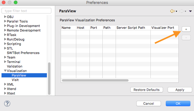
- Windows or Linux: in ICE's toolbar, select Window > Preferences, then Visualization > ParaView in the tree of the "Preferences" page.
- Mac OS X: in ICE's toolbar, select ICE > Preferences, then Visualization > ParaView in the tree of the "Preferences" page.
Press the new row button (stylized as a "+" symbol) in the upper-right corner of the resulting dialog box.
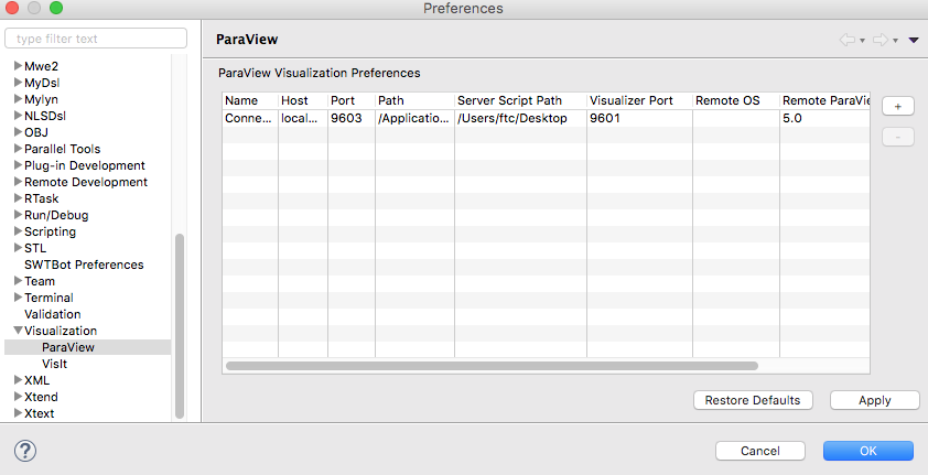
ICE automatically supplies some, but not all, parameters when adding a ParaView connection (e.g., the user will need to specify their http_pvw_server.py path). Below is a list of parameters required (unless otherwise noted) for full ParaView functionality in a given configuration.
- Host: The default value for this field is "localhost," which is used for connecting to a local installation of ParaView on a user's machine; keep this setting if you are running ParaView on the same machine as the ICE framework. To launch a remote ParaView connection, the remote hostname/address should be entered into this field.
- Path: If correctly installed, the ParaView path should populate in ICE by default. If not, the user should add the full path to the local ParaView installation. The path should end with the folder containing the ParaView executable.
- On a Windows machine, the path will be based on where you extracted the contents of the ParaView-5.2.0-Qt4-OpenGL2-Windows-64bit.zip archive. For example, if you unzipped to the desktop without renaming the archive, the path would be:
- C:\Users\[UserName]\Desktop\ParaView-5.2.0-Qt4-OpenGL2-Windows-64bit\
- On a Linux machine, the path will be based on where you extracted the contents of the ParaView-5.2.0-Qt4-OpenGL2-MPI-Linux-64bit.tar.gz archive. For example, if you unzipped to the desktop without renaming the archive, the path would be:
- /home/[UserName]/Desktop/ParaView-5.2.0-Qt4-OpenGL2-MPI-Linux-64bit/
- On Mac OS X, ParaView's executable should be installed in the machine's "Applications" directory, unless otherwise specified by the user. Therefore, the path would simply be:
- /Applications/
- On a Windows machine, the path will be based on where you extracted the contents of the ParaView-5.2.0-Qt4-OpenGL2-Windows-64bit.zip archive. For example, if you unzipped to the desktop without renaming the archive, the path would be:
- Server Script Path: The full path to the http_pvw_server.py file, ending with the folder containing it. For example, if the file is on your desktop, the path might be:
- Windows: C:\Users\[UserName]\Desktop\
- Linux: /home/[UserName]/Desktop/
- Mac OS X: /Users/[UserName]/Desktop/
- Port: The default port number for ParaView is 9600. However, if you are using both VisIt and ParaView within ICE, this value should differ for each application, and this number needs to be changed to avoid connection errors (e.g., from 9600 to 9603 for ParaView).
- Web Visualizer Port: The default port number for the ParaView web visualizer is 9601. If changed, it must differ from the ParaView (and VisIt) port number.
- Remote OS: The operating system of the remote machine on which ParaView will be launched. If you are launching ParaView on your local machine, ignore this cell.
- Remote ParaView Version Number: The version of ParaView you are using. This may be ignored unless you are launching a remote ParaView session on a Linux machine. You can check your installation's version number by looking inside the top level lib directory. The lib directory should contain a folder named paraview- followed by the version number.
Once finished, click Apply, and then click OK. ICE will then launch a ParaView session.
If you are connecting to a remote host, you may be prompted to "allow" the connection to the remote host. Click Yes to trust the connection, and enter the credentials for the remote machine in the prompt.
ParaView Plot Editor
Once a connection with ParaView has been established, the "Plot Editor" view will appear and display the contents of the file that was imported into "Project 1." This view allows the user to manipulate the visualization just as they would with the ParaView GUI.
If at any point you should close the "Plot Editor," simply double click on the imported file to redraw the visualization.
A ParaView plot editor will allow you to choose the mesh and scalar to be modeled and to choose the model's representation. These editors also feature a slider at the bottom, allowing the user to interact with time data.
The arrow buttons move to the previous or next time step, and the triangle button enables the "Plot Editor" to play the simulation automatically. The last button on the right displays playback options.
The visualization's current time step is also displayed, and you can manually drag the slider along the timeline to choose a specific time step to display.
The ParaView plot editor also has a Launch in Web Visualizer button to open the file in ParaView's Web Visualizer inside of ICE. The full functionality of the Web Visualizer is beyond the scope of this article, but interested readers can learn more from the official documentation.
CSV Plot Tools
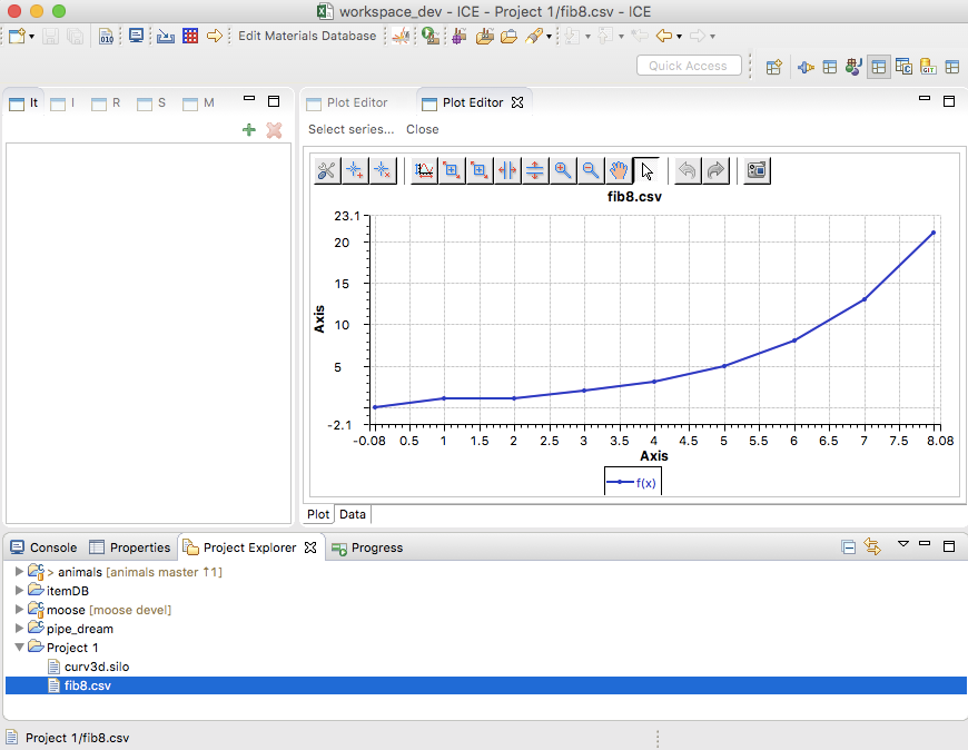
Unlike VisIt and ParaView, no connection configuration is necessary for launching a CSV visualization session. Out of the box, ICE includes basic CSV data-plotting utilities for fast and easy x, y graph visualizations. This section describes how to open your .csv data files from the "Project Explorer" and render them in the "Plot Editor."
First, add your .csv data file to the "Project Explorer" (see Adding the Data File) using the Import button in the ICE toolbar.
Next, double click the newly-imported .csv file as it appears in your "Project Explorer" (fib8v.csv in this example) to render the visualization in the "Plot Editor."
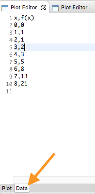
The user can also edit the .csv within ICE by clicking on the Data tab in the "Plot Editor" view.
Selecting a Series
By default, the first series in the file will be used as the independent variable (used to determine the x-axis values of all points), and the second series is graphed as a dependent variable. Both can be changed.
Changing the Independent Variable
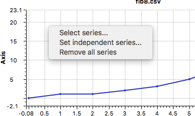
To set the independent (variable) series, right click in the Plot Editor and select Set independent series...
In the resulting dialog, make your selection, and click OK.
Changing the Graphed Series
There are two ways to select the graphed series.
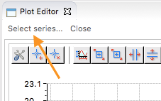
1. Graph a single series, removing all others. Click the Select series... button in the upper left corner.
Choose which series to graph by making the appropriate selection in the resulting dialog window. Click OK.
2. Graph multiple series. Right click in the Plot Editor, then click Select series... within the resulting context menu.
Choose which series to graph by selecting the appropriate check boxes in the resulting dialog window. After making a selection, click OK.
You can also remove all graphed series by right clicking in the "Plot Editor" and choosing Remove all series.
Plot Toolbar
The plotting widget used by ICE's CSV "Plot Editor" includes a toolbar with helpful utilities for navigating your plotted data or customizing the plot's appearance. You can hover over each button with your cursor to view a tool tip describing what each button does.
Clicking the first button will open a dialog that allows you to customize the appearance of the plot or individual series on the plot—including titles, scales, grids, colors, and fonts. The last button allows you to save the current plot as a .png image file. Feel free to try out the different utilities available in this toolbar.

