Transportation Models

Mixing Between Adjacent Regions in Spatiotemporal Models

The Introduction to Compartment Models describes how an infectious disease evolves in time. STEM also allows users to represent the geographic distribution of people (or animals) and how they move about in space. A compartment model that deals only with the trajectory of a disease in time implicitly assumes that the population (or populations) in question is so well mixed that there is no need to model the spatial distribution of people. However, for very large scale simulations, the details of population distribution, transportation, trade, even wild bird migration can all be important factors in understanding the evolution of an infectious disease in space and time. The following page describes how Transportation Models are implemented in STEM.

As a convenience to users STEM implements a simple nearest neighbor mixing models for human populations based on the existing common border edges in the built in graphs in STEM. Common Border edges represent physical adjacency. The default mixing model can be disabled by setting a mixing distance, &lamda; to zero. The default mixing model is described below. Please note, if a user defines any custom mixing edges within their graph, the default mixing model is not used and only the user defined mixing is invoked.

Default Mixing Model

Without going into the complete details of a Spatiotemporal Compartment model, let’s look at the interaction term defined in equation <1a>. Imagine that this equation is being used to define the rate at which infectious people at some particular location j cause susceptible people at the same location j to become infectious. We might then write the same equation as:

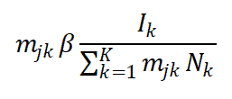
Let the rate of infection in the population j form mixing with population k be:

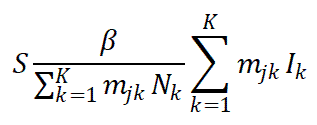
Then the rate of new infections (incidence rate) in population j is:

where:

mjk is the mixing rate between j and k (note that mjj=1 )
Ik is the number of infectious in population k
K is the total number of populations
Nk is the population in patch k
β is the transmission coefficient

Under these assumptions, the within patch reproductive number is:

where the sum is taken over all sites k. The vectors that connect different locations are represented by the set of m_jk. Connections need not be only between adjacent locations. For example, air travel map provide connections between distant sites.

Today STEM disease models use several types of edges to model transportation.

• Common Border Edges with Common Border Labels are used to compute the circulation of people between neighbors by mixing as described above. 
  Common Border Edges are based only on geometrical and geographic facts.
• Road Transportation Edges are connections weighted by the number of roads connecting two regions.
• Air Transportation Edges represent transportation by Air Travel.

In the future STEM will also provide edges that model motion specific to particular populations or species. These new Mixing and Migration'' Edges will associate a transportation rate with the population by name.

• Mixing Edges represent circulation of the population with each edge associated with a particular population by name. Today this is done with (bidirectional) Common Border Edges (and the computation simply assumes a human population).
• Migration Edges represent migration of people over time. With these directed edges, users can specify migration rates or create their own migration model.

Mixing Approximations

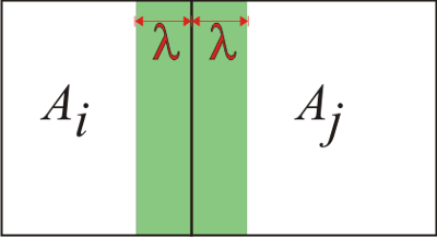
Not all administrative regions are the same size. The STEM model for mixing or circulation of a population scales the mixing rate by an effective depth  λ for each region. This is analogous assuming a skin depth or average mixing length scale. The figure below shows a simple example of two adjacent nearly square regions of area A_i and A_j respectively.

Today STEM uses the simplest possible approximation for the characteristic mixing in this model, the fraction of people leaving site j for any neighboring site i becomes:

Where the average mixing length, 𝜆_o, is determined as part of an optimization process. Typically we find 𝜆o ≲ 45km.

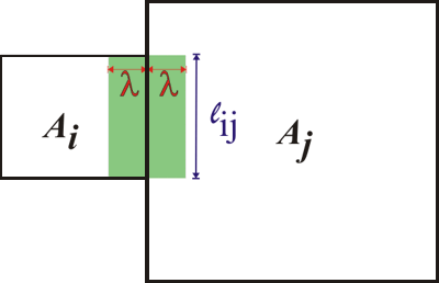
In reality, the polygons in STEM are quite varied in shape. The figure below shows two adjacent regions (again with simple shapes) associated with a common border of length ℓ_ij

In this example a better approximation for the fraction of people leaving site j for any neighboring site k is given by:

The STEM Common Border edge data sets now include the correct common border length, ℓij, for each edge. Since version 1.4, STEM uses the better approximation taking into account the common border length.

Custom Mixing Models: Mixing Edges

Advanced users may optionally define their own model of mixing. A user-defined mixing model can be implemented by creating a custom set of special "mixing edges" and adding it to the user's graph. For convenience STEM provides a mixing edge graph generator that will generate a set of mixing edges based on the common border edges already defined in the user's graph. Mixing edges are non-directed. Mixing edges have the following properties:

• Mixing Rate
• useAbsoluteValues (a boolean) to indicate if the rate is a fraction of the population (default) or an absolute count or number mixing in the default time step
• Population, a string that labels the population mixing (e.g., human, cattle, etc.)
• NodeA <=> NodeB

The mixing edge graph generator creates the graph of mixing edges with a user-specified default value. Users are free to edit the (generated) .graph file and specify individual rates for each mixing edge. The advantage to a custom mixing model is its transparency (each edge lists its mixing rate). The disadvantage is that it is up to the user to define these rates or to implement an algorithm to set or reset them. IF a user graph contains ANY custom mixing edges, STEM will NOT iterate the default internal mixing model described above.

Migration Between Regions

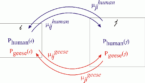
Unlike population mixing which modifies the terms in a disease model computation, migration is a property of the population itself. The figure below shows a simple example with two locations, i & j , each containing a population of humans and a population of geese.

Migration Edges are directed. There is one edge for each direction of migration (i=>j and j=>i). Migration edges are also specific to the population type (humans or geese in this example) and, of course, they are labeled by a migration rate μ which represents the fraction of the population that moves from one site to another in a given time period (usually one day). In general, μ_ij≠μ_ji. When they are not equal there is a net migration of the population form one node to the other. If the migration rates are equal then the populations are mixing (and user can consider using mixing edges for this purpose).

Today STEM provides a tool to generate a graph of migration edges for an existing lattice graph. In the future new tools will be provided including a graphical editor to allow creation of specific edges and a function to import a graph from a user-defined file.